Implementing the Generator in Python

Understanding the Generator Architecture

Unveiling the Discriminator

Coding the Discriminator in Python

Decoding the Discriminator Architecture

Testing Discriminator

Loading Real Data (Test Images MNIST)

The Dance Begins: Training Your GAN

Vanilla GAN

How it all works

Results

Training GANs: Challenges and Solutions

Improving GAN Training Stability

Evaluating GAN Performance

Things to Try

Chapter 04 Chapter 4: Building Your First GAN

Buckle up and rev your engines because we're diving headfirst into the wild world of Generative Adversarial Networks (GANs)! With Python as your trusty sidekick, you'll conquer GANs and create mind-blowing art, music, and images that'll make your jaw drop. So, let's fire up your code editor, grab a cup of coffee (or your favourite drink), and get ready to make some magic happen!

Let's do a simple test to make sure pytorch is installed and ready. You'll print out the version:

>>> import torch
>>> print(torch.__version__)
2.1.0.dev20230704+cu121

Vanilla GANs

The three main parts to the Vanilla GAN, are:

Generator
Discriminator
Trainer

The Generator uses a fully connected network, i.e., Sequential(.. Linear(..) )`.

Creating the Generator

Start by implementing a vanilla generator for a small image (28x28 gray scale image). The input will be a random vector (dimensions 64). You'll add a number of constants at the top to represent common variables that will be used in multiple places.

Implementing the Generator in Python

import os
import torch
from torch import nn

# Configurable variables
NOISE_DIMENSION = 64
GENERATOR_OUTPUT_IMAGE_SHAPE = 28 * 28 * 1

"""
Vanilla GAN Generator
"""
G = nn.Sequential(
      # First upsampling
      nn.Linear(NOISE_DIMENSION, 128, bias=False),
      nn.LeakyReLU(0.25),
      # Second upsampling
      nn.Linear(128, 256, bias=False),
      nn.LeakyReLU(0.25),
      # Third upsampling
      nn.Linear(256, 512, bias=False),
      nn.LeakyReLU(0.25),
      # Final upsampling
      nn.Linear(512, GENERATOR_OUTPUT_IMAGE_SHAPE, bias=False),
      nn.Tanh()
    )

It doesn't do much, and you'll want to make sure it works! Create a small test setup that inputs some random noise and draws the output on screen.

Batch normalization (also known as batch norm) is a method used to make training of artificial neural networks faster and more stable through normalization of the layers' inputs by re-centering and re-scaling.

Since batch normalization requires an array of images, for testing, so you can create a single image, you'll comment out the batch normalization sections.

import os
import torch
from torch import nn
import numpy as np
import matplotlib.pyplot as plt

# Configurable variables
NOISE_DIMENSION = 64
GENERATOR_OUTPUT_IMAGE_SHAPE = 28 * 28 * 1
BATCH_SIZE = 128

# Device configuration (GPU or CPU)
device = torch.device('cuda' if torch.cuda.is_available() else 'cpu')

"""
Vanilla GAN Generator
"""
G = nn.Sequential(
      # First upsampling
      nn.Linear(NOISE_DIMENSION, 128, bias=False),
      nn.LeakyReLU(0.25),
      # Second upsampling
      nn.Linear(128, 256, bias=False),
      nn.LeakyReLU(0.25),
      # Third upsampling
      nn.Linear(256, 512, bias=False),
      nn.LeakyReLU(0.25),
      # Final upsampling
      nn.Linear(512, GENERATOR_OUTPUT_IMAGE_SHAPE, bias=False),
      nn.Tanh()
    ).to(device)



# -------- Test Generator -----------
""" Generate noise for number_of_images images, with a specific noise_dimension """
z = torch.randn(1 , # BATCH_SIZE, # number_of_images, 
                NOISE_DIMENSION, # noise_dimension
                device=device)
fake = G(z)

""" Display the fake image from the generator """ 
generated_image = G(z).reshape(28, 28).detach().cpu().numpy()
plt.imshow(generated_image, cmap='gray')
plt.axis('off')
plt.savefig(f'generated_image.png')
plt.close()

The output is what you'd expect, random 28x28 pixel image:

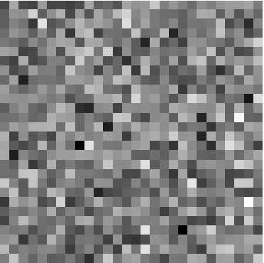
As you'll start to train the network weights it will create images that emulate the properties of the real images you'll use for training.

The last activation function is nn.Tanh() so the generated pixel colors are in the range -1 to 1. When saving or displaying the image you'll need to convert them to 0 to 256 unsigned int.

Understanding the Generator Architecture

The generator neural network using PyTorch's nn.Sequential module. The generator is designed to create synthetic data (images) using a random noise vector as input. Let's break down the code step by step:

nn.Sequential: This is a container for a sequence of neural network modules, where the output of each module is fed as the input to the next one in the sequence.
nn.Linear(NOISE_DIMENSION, 128, bias=False): This line creates the first layer of the generator. It is a fully connected (dense) layer that takes input of size NOISE_DIMENSION and produces an output of size 128. The bias=False argument means that there are no bias terms added to the layer.
nn.LeakyReLU(0.25): After each linear layer, a Leaky Rectified Linear Unit (ReLU) activation function is applied. Leaky ReLU is a variant of the standard ReLU activation, which allows a small negative slope (defined as 0.25 in this case) for the negative inputs, preventing the issue of "dying ReLU" and promoting better gradient flow during training.
nn.Linear(128, 256, bias=False): The second fully connected layer takes the output of the previous layer (size 128) and produces an output of size 256.
nn.LeakyReLU(0.25): The second Leaky ReLU activation function is applied.
nn.Linear(256, 512, bias=False): The third fully connected layer takes the output of the previous layer (size 256) and produces an output of size 512.
nn.LeakyReLU(0.25): The third Leaky ReLU activation function is applied.
nn.Linear(512, GENERATOR_OUTPUT_IMAGE_SHAPE, bias=False): The final fully connected layer takes the output of the previous layer (size 512) and produces an output of size GENERATOR_OUTPUT_IMAGE_SHAPE. This layer's purpose is to map the high-dimensional feature space to the desired output space, which is the image space in this case.
nn.Tanh(): The last activation function used in the generator is the hyperbolic tangent (tanh) function. The tanh function squashes the output values to the range [-1, 1], which is common for image data as the pixel values are usually scaled to this range. It's used to ensure that the output image is appropriately scaled.
.to(device): This line moves the entire generator model to a specific device (e.g., GPU) if available. This is commonly done to accelerate computation on hardware accelerators like GPUs.

The generator neural network with several fully connected layers, each followed by a Leaky ReLU activation function, to transform a random noise vector (of size NOISE_DIMENSION) into a synthetic image (of shape GENERATOR_OUTPUT_IMAGE_SHAPE). This generator is often used in Generative Adversarial Networks (GANs) or other generative models to create synthetic data that resembles the real data distribution.

Unveiling the Discriminator

The discriminator is very simple, you give it some data, and it returns true or false (is the data real or fake).

Coding the Discriminator in Python

"""
Vanilla GAN Discriminator
"""
D = nn.Sequential(
    nn.Linear(GENERATOR_OUTPUT_IMAGE_SHAPE, 1024), 
    nn.LeakyReLU(0.25),
    nn.Linear(1024, 512), 
    nn.LeakyReLU(0.25),
    nn.Linear(512, 256), 
    nn.LeakyReLU(0.25),
    nn.Linear(256, 1),
    nn.Sigmoid()
).to(device)

Decoding the Discriminator Architecture

This code defines a discriminator neural network using PyTorch's nn.Sequential module. The discriminator is a binary classifier that takes an input image and determines whether it is real (belonging to the real dataset) or fake (generated by the generator).

Let's break down the discriminator code step by step:

nn.Sequential: Similar to the generator code you provided earlier, this is a container for a sequence of neural network modules, where the output of each module is fed as the input to the next one in the sequence.
nn.Linear(GENERATOR_OUTPUT_IMAGE_SHAPE, 1024): The first layer of the discriminator is a fully connected (dense) layer that takes an input image of size GENERATOR_OUTPUT_IMAGE_SHAPE (the same shape as the output of the generator) and produces an output of size 1024.
nn.LeakyReLU(0.25): After each linear layer, a Leaky Rectified Linear Unit (ReLU) activation function is applied. Leaky ReLU is used to introduce a small negative slope (defined as 0.25 in this case) for negative inputs, which helps prevent the "dying ReLU" problem and provides better gradient flow during training.
nn.Linear(1024, 512): The second fully connected layer takes the output of the previous layer (size 1024) and produces an output of size 512.
nn.LeakyReLU(0.25): The second Leaky ReLU activation function is applied.
nn.Linear(512, 256): The third fully connected layer takes the output of the previous layer (size 512) and produces an output of size 256.
nn.LeakyReLU(0.25): The third Leaky ReLU activation function is applied.
nn.Linear(256, 1): The final fully connected layer takes the output of the previous layer (size 256) and produces an output of size 1. This is the final output of the discriminator, and it represents the probability that the input image is real.
nn.Sigmoid(): The last activation function used in the discriminator is the sigmoid function. The sigmoid function maps the output to a value between 0 and 1, representing the probability that the input image is real (1 for real and 0 for fake).
.to(device): This line moves the entire discriminator model to a specific device (e.g., GPU) if available. Similar to the generator, this is commonly done to accelerate computation on hardware accelerators like GPUs.

The discriminator neural network with several fully connected layers, each followed by a Leaky ReLU activation function. The discriminator takes an input image (generated by the generator) and produces an output value between 0 and 1, representing the probability that the input image is real (1 for real images and 0 for fake images). The discriminator is trained to distinguish between real and fake images and is a crucial part of the Generative Adversarial Network (GAN) architecture, where it competes with the generator in a two-player minimax game to improve the overall quality of the generated images.

Testing Discriminator

Very easy to check that your discriminator is running by passing it the output from the generator or a real image. The result should be a single value (how real or fake the discriminator thinks the data is). Of course, it hasn't been trained yet, so the value will be arbitrary, but still, it lets you see that the code is doing what it should (no errors and you get an output).

import os
import torch
from torch import nn
import numpy as np
import matplotlib.pyplot as plt

# Configurable variables
NOISE_DIMENSION = 64
GENERATOR_OUTPUT_IMAGE_SHAPE = 28 * 28 * 1
BATCH_SIZE = 128

# Device configuration (GPU or CPU)
device = torch.device('cuda' if torch.cuda.is_available() else 'cpu')

"""
Vanilla GAN Generator
"""
G = nn.Sequential(
      # First upsampling
      nn.Linear(NOISE_DIMENSION, 128, bias=False),
      nn.LeakyReLU(0.25),
      # Second upsampling
      nn.Linear(128, 256, bias=False),
      nn.LeakyReLU(0.25),
      # Third upsampling
      nn.Linear(256, 512, bias=False),
      nn.LeakyReLU(0.25),
      # Final upsampling
      nn.Linear(512, GENERATOR_OUTPUT_IMAGE_SHAPE, bias=False),
      nn.Tanh()
    ).to(device)

"""
Vanilla GAN Discriminator
"""
D = nn.Sequential(
    nn.Linear(GENERATOR_OUTPUT_IMAGE_SHAPE, 1024), 
    nn.LeakyReLU(0.25),
    nn.Linear(1024, 512), 
    nn.LeakyReLU(0.25),
    nn.Linear(512, 256), 
    nn.LeakyReLU(0.25),
    nn.Linear(256, 1),
    nn.Sigmoid()
).to(device)


# -------- Test Generator -----------
""" Generate noise for number_of_images images, with a specific noise_dimension """
z = torch.randn(1 , # BATCH_SIZE, # number_of_images, 
                NOISE_DIMENSION, # noise_dimension
                device=device)

fake = G(z)


# -------- Test Descriminator -------

test = D(fake) # <<-----

print( test ); # <<----- e.g., 0.458

Loading Real Data (Test Images MNIST)

In addition to generating fake data using our generator, you'll also need some real data.

You'll take advantage of the MNIST dataset, which provides a library of hand written numbers. Very easy to load and use with the torchvision library. You can load the data set in with a few lines of code.

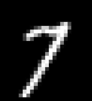
The following code show a simplified example that loads in the dataset and display one of the images.

import os
import torch
from torch.utils.data import DataLoader
from torchvision import datasets, transforms
import matplotlib.pyplot as plt

# Configurable variables
BATCH_SIZE = 128

# MNIST dataset
dataset = datasets.MNIST(root='data', train=True, transform=transforms.ToTensor(), download=True)            
data_loader = DataLoader(dataset=dataset, batch_size=BATCH_SIZE, shuffle=True)


data_iterator = iter(data_loader)
images, labels = next(data_iterator)

image = images[0]
image_np = image.squeeze().numpy()

plt.imshow(image_np, cmap='gray')
plt.axis('off')
plt.show()

You can see an example of the output below (drawn image on a black background).

The Dance Begins: Training Your GAN

This is were we bring things together, output from the generator, loaded real data and the discriminators result (which was real).

Vanilla GAN

Below is the combined implementation with a training loop. The results after a 5 minute run (5000 iterations) isn't bad:

import os
import torch
from torch import nn
import torch.optim as optim
from torch.utils.data import DataLoader
from torchvision import datasets, transforms
import matplotlib.pyplot as plt
import numpy as np

# Configurable variables
NOISE_DIMENSION = 64
GENERATOR_OUTPUT_IMAGE_SHAPE = 28 * 28 * 1
BATCH_SIZE = 128
LEARNING_RATE = 0.0002
NUM_EPOCHS = 5000

# Device configuration (GPU or CPU)
device = torch.device('cuda' if torch.cuda.is_available() else 'cpu')

"""
MNIST dataset (28x28 gray scale images)
"""
dataset = datasets.MNIST(root='data', train=True, transform=transforms.ToTensor(), download=True)            
data_loader = DataLoader(dataset=dataset, batch_size=BATCH_SIZE, shuffle=True)

"""
Vanilla GAN Generator
"""
G = nn.Sequential(
      # First upsampling
      nn.Linear(NOISE_DIMENSION, 128, bias=False),
      nn.LeakyReLU(0.25),
      # Second upsampling
      nn.Linear(128, 256, bias=False),
      nn.LeakyReLU(0.25),
      # Third upsampling
      nn.Linear(256, 512, bias=False),
      nn.LeakyReLU(0.25),
      # Final upsampling
      nn.Linear(512, GENERATOR_OUTPUT_IMAGE_SHAPE, bias=False),
      nn.Tanh()
    ).to(device)  

"""
Vanilla GAN Discriminator
"""
D = nn.Sequential(
    nn.Linear(GENERATOR_OUTPUT_IMAGE_SHAPE, 1024), 
    nn.LeakyReLU(0.25),
    nn.Linear(1024, 512), 
    nn.LeakyReLU(0.25),
    nn.Linear(512, 256), 
    nn.LeakyReLU(0.25),
    nn.Linear(256, 1),
    nn.Sigmoid()
).to(device)


# Loss and optimizer
criterion = nn.BCELoss()
d_optimizer = optim.Adam(D.parameters(), lr=LEARNING_RATE)
g_optimizer = optim.Adam(G.parameters(), lr=LEARNING_RATE)


for epoch in range(0,NUM_EPOCHS):
    data_iterator = iter(data_loader)
    images, labels = next(data_iterator)

    batch_size = images.size(0)
    images = images.reshape(batch_size, -1).to(device)

    # Labels for real and fake images
    real_labels = torch.ones(batch_size, 1).to(device)
    fake_labels = torch.zeros(batch_size, 1).to(device)

    # Training the discriminator
    # Real images
    outputs = D(images)
    d_loss_real = criterion(outputs, real_labels)
    real_score = outputs

    # Fake images
    z = torch.randn(batch_size, NOISE_DIMENSION).to(device)
    fake_images = G(z)
    outputs = D(fake_images.detach())
    d_loss_fake = criterion(outputs, fake_labels)
    fake_score = outputs

    # Total discriminator loss
    d_loss = d_loss_real + d_loss_fake

    d_optimizer.zero_grad()
    g_optimizer.zero_grad()
    d_loss.backward()
    d_optimizer.step()

    # Training the generator
    z = torch.randn(batch_size, NOISE_DIMENSION).to(device)
    fake_images = G(z)
    outputs = D(fake_images)
    g_loss = criterion(outputs, real_labels)

    d_optimizer.zero_grad()
    g_optimizer.zero_grad()
    g_loss.backward()
    g_optimizer.step()

    if epoch % 100 == 0:
        print(f"Epoch [{epoch+1}/{NUM_EPOCHS}], Step [{epoch}/{len(data_loader)}], "
              f"D_loss: {d_loss.item():.4f}, G_loss: {g_loss.item():.4f}, "
              f"D(x): {real_score.mean().item():.2f}, D(G(z)): {fake_score.mean().item():.2f}")



""" 
Display the fake image from the generator 
""" 
generaged_images = G(z)[0]
generated_image = generaged_images.reshape(28, 28).detach().cpu().numpy()
plt.imshow(generated_image, cmap='gray')
plt.axis('off')
plt.savefig(f'generated_image.png')
plt.close()

Label Smoothing Notice the labels for the real and fake use 1.0 and 0.0. However, a concept called label smoothing adds a small amount of randomness to the values (e.g., instead of 1.0 it would be between 0.9 and 1.1). This effects the training times and image quality.

How it all works

This code implements a Vanilla Generative Adversarial Network (GAN) using PyTorch to generate synthetic images resembling the MNIST dataset's handwritten digits. The GAN consists of a generator (G) and a discriminator (D). The generator generates fake images, and the discriminator tries to distinguish between real and fake images.

Let's break down the code and understand what each part does:

Imports: The code imports various necessary libraries such as PyTorch (torch), neural network modules (nn), optimization functions (optim), data utilities (DataLoader), MNIST dataset (datasets), data transformations (transforms), plotting library (matplotlib.pyplot), and NumPy (numpy).
Configurable Variables: These variables define the hyperparameters of the GAN, such as the noise dimension (NOISE_DIMENSION), image shape for the generator's output (GENERATOR_OUTPUT_IMAGE_SHAPE), batch size (BATCH_SIZE), learning rate (LEARNING_RATE), and the number of epochs to train (NUM_EPOCHS).
Device Configuration: The code determines whether to use a GPU (cuda) if available, otherwise, it will fall back to using the CPU.
MNIST Dataset: The code loads the MNIST dataset, applies a ToTensor() transformation to convert the images to PyTorch tensors, and creates a data loader to efficiently handle batches during training.
Vanilla GAN Generator: The generator G is defined using a sequence of fully connected layers (nn.Linear) interspersed with leaky ReLU activation functions (nn.LeakyReLU) and a final Tanh() activation function. The generator takes a noise vector of size NOISE_DIMENSION as input and outputs synthetic images of shape GENERATOR_OUTPUT_IMAGE_SHAPE. It is moved to the selected device using .to(device).
Vanilla GAN Discriminator: The discriminator D is defined similarly to the generator, but it uses larger fully connected layers. The discriminator takes an image as input (flattened to a vector) and outputs a single value between 0 and 1, representing the probability that the input image is real. It is moved to the selected device using .to(device).
Loss and Optimizer: The code defines the binary cross-entropy loss (BCELoss) and two Adam optimizers for both the discriminator (d_optimizer) and the generator (g_optimizer).
Training Loop: The code runs a loop for NUM_EPOCHS epochs. In each epoch, it iterates through the data loader to get real images from the MNIST dataset.
Discriminator Training: The discriminator is trained to distinguish between real and fake images. It calculates the loss for real images and fake images separately, and then backpropagates the gradients to update the discriminator's parameters.
Generator Training: The generator is trained to generate images that can fool the discriminator into classifying them as real. It calculates the generator loss and backpropagates the gradients to update the generator's parameters.
Printing Progress: Every 100 epochs, the code prints the current epoch, discriminator loss (D_loss), generator loss (G_loss), mean score of real images (D(x)), and mean score of fake images (D(G(z))).

As the training progresses, the generator learns to produce more realistic images, while the discriminator improves its ability to differentiate between real and fake images.

Over time, the quality of the generated image should improve, and the discriminator becomes more adept at distinguishing real images from the synthetic ones.

Key points:

The GAN Training Process: Minimax Game (real or fake)
Loss functions: Binary Cross-Entropy, Wasserstein Loss
Optimization techniques: Adam (try others such as, RMSprop, SGD)
Fixed learning rate, but you can monitor and fine-tune this for more optimal results

Results

The output from the vanilla GAN isn't too bad.

Training GANs: Challenges and Solutions

Once you've got your GAN up and running, you'll want to do some tinkering, trying to improve the image quality, training times and so on.

Improving GAN Training Stability

In the vanilla example, you'll find that the output actually converges on something that looks like the real data. However, there can be situations, when your output never converges or it converges then goes off and gets lost!

Evaluating GAN Performance

There are many measures of performance, the key ones are:

Number of epochs to achieve an acceptable solution
Percentage of real vs fake

Things to Try

Lists some ideas for extending and exploring the Vanilla GAN solution provided in this chapter.

Try alternative activation and scaling (e.g., Tanh activation function generates pixel values in the range [-1,1], but you can try other activation functions and ranges.
Random number input for the generator (a.k.a. Latent Space). Try larger or smaller input ranges (e.g., 32 random numbers vs 512) and compare the quality of the results and speed of training. Also try out different random number generators (quality/distribution of the randomness)
Different model configurations, such as, deeper or more shallow discriminator and/or generator networks, perhaps experiment with the UpSampling2D layers
in the generator.