Chapter 05 Chapter 5: DCGAN: Deep Convolutional GANs

DCGAN, or Deep Convolutional GAN, is a generative adversarial network architecture. It uses a couple of guidelines, in particular: Replacing any pooling layers with strided convolutions (discriminator) and fractional-strided convolutions (generator). Using batchnorm in both the generator and the discriminator.

Deep Convolutional Networks

Convolutions are not densely connected, not all input nodes affect all output nodes. This gives convolutional layers more flexibility in learning. Moreover, the number of weights per layer is a lot smaller, which helps a lot with high-dimensional inputs such as image data.

Shake things up a little by using a different dataset (color images). Instead of single grayscale 1x28x28 (MNIST), you'll use 3x64x64 set of color images (Celeb dataset).

CelebA Image Dataset

What Is CelebA? CelebFaces Attributes Dataset, or CelebA for short, is an image dataset that identifies celebrity face attributes. It contains 202,599 face images across five landmark locations, with 40 binary attribute annotations for each image. It currently includes data relating to over 10,000 celebrities.

# Root directory for the dataset
import torchvision.datasets 
data_root = 'data/celeba'
# Spatial size of training images, images are resized to this size.
image_size = 64

celeba_data = torchvision.datasets.CelebA(root=data_root,
                              download=True,
                              transform=transforms.Compose([
                                  transforms.Resize(image_size),
                                  transforms.CenterCrop(image_size),
                                  transforms.ToTensor(),
                                  transforms.Normalize(mean=[0.5, 0.5, 0.5],
                                                       std=[0.5, 0.5, 0.5])
                              ]))

"Google Drive - Quota exceeded". This time it returns RuntimeError('Dataset not found or corrupted.'

Custom Dataset Downloader

import os
import zipfile 
import gdown
import torch
from natsort import natsorted
from PIL import Image
from torch.utils.data import Dataset
from torchvision import transforms
import matplotlib.pyplot as plt


## Create a custom Dataset class
class CelebADataset(Dataset):
  def __init__(self, root_dir, transform=None):

    # Create required directories 
    if not os.path.exists(root_dir):
        os.makedirs(root_dir)

    # Path to download the dataset to    
    download_path = f'{root_dir}/img_align_celeba.zip'
    if not os.path.exists(download_path):
        ## Fetch data from url 
        # URL for the CelebA dataset
        url = 'https://s3-us-west-1.amazonaws.com/udacity-dlnfd/datasets/celeba.zip'

        # Download the dataset from google drive
        gdown.download(url, download_path, quiet=False)

        # Unzip the downloaded file 
        with zipfile.ZipFile(download_path, 'r') as ziphandler:
            ziphandler.extractall(root_dir)

    # Read names of images in the root directory
    image_names = os.listdir(root_dir + '/img_align_celeba/')

    self.root_dir = root_dir + '/img_align_celeba/'
    self.transform = transform 
    self.image_names = natsorted(image_names)
    # print('self.image_names:', self.image_names )

  def __len__(self): 
    return len(self.image_names)

  def __getitem__(self, idx):
    # Get the path to the image 
    img_path = os.path.join(self.root_dir, self.image_names[idx])
    # Load image and convert it to RGB
    img = Image.open(img_path).convert('RGB')
    # Apply transformations to the image
    if self.transform:
      img = self.transform(img)

    return img

## Load the dataset 
# Path to directory with all the images
img_folder = 'data/celeba/img_align_celeba'
# Spatial size of training images, images are resized to this size.
image_size = 64
# Transformations to be applied to each individual image sample
transform=transforms.Compose([
    transforms.Resize(image_size),
    transforms.CenterCrop(image_size),
    transforms.ToTensor(),
    transforms.Normalize(mean=[0.5, 0.5, 0.5],
                          std=[0.5, 0.5, 0.5])
])

# Load the dataset from file and apply transformations
celeba_dataset = CelebADataset(img_folder, transform)

batch_size = 128
num_workers = 0
pin_memory = 0

celeba_dataloader = torch.utils.data.DataLoader(celeba_dataset,
                                                batch_size=batch_size,
                                                num_workers=num_workers,
                                                pin_memory=pin_memory,
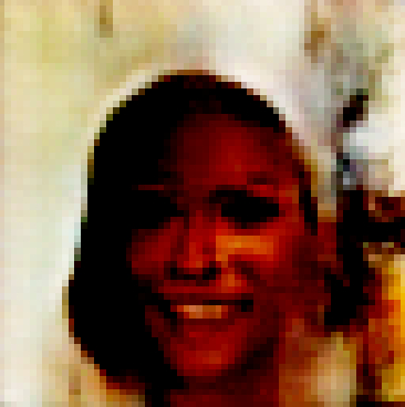
                                                shuffle=True)

Add a few extra lines to test the loader to show one of the celeb pictures:

data_iterator = iter(celeba_dataloader)
images = next(data_iterator)

image = images[0]
image_np = image.permute(1, 2, 0).numpy()

plt.imshow(image_np)
plt.axis('off')
plt.show()

Instead of using torchvision.datasets.CelebA(..), you'd use CelebADataset(..).

Generator

The DCGAN generator consists of multiple layers of transposed convolutions, batch normalization, and ReLU activation functions, progressively upsampling from a 100-dimensional noise input to a 3-channel output image with a resolution of 64x64 pixels, followed by a Tanh activation to map pixel values between -1 and 1.

G = nn.Sequential(
    # Input is 100, going into a convolution.
    nn.ConvTranspose2d(NOISE_DIMENSION, 512, (4, 4), (1, 1), (0, 0), bias=False),
    nn.BatchNorm2d(512),
    nn.ReLU(True),
    # state size. 512 x 4 x 4
    nn.ConvTranspose2d(512, 256, (4, 4), (2, 2), (1, 1), bias=False),
    nn.BatchNorm2d(256),
    nn.ReLU(True),
    # state size. 256 x 8 x 8
    nn.ConvTranspose2d(256, 128, (4, 4), (2, 2), (1, 1), bias=False),
    nn.BatchNorm2d(128),
    nn.ReLU(True),
    # state size. 128 x 16 x 16
    nn.ConvTranspose2d(128, 64, (4, 4), (2, 2), (1, 1), bias=False),
    nn.BatchNorm2d(64),
    nn.ReLU(True),
    # state size. 64 x 32 x 32
    nn.ConvTranspose2d(64, 3, (4, 4), (2, 2), (1, 1), bias=True),
    nn.Tanh()
    # state size. 3 x 64 x 64
).to(device) 

Testing Generator (RGB Output)

Obviously, the generator is only going to produce noise, but it's a nice step just to check it's working.

# -------- Test Generator -----------
""" Generate noise input """
z = torch.randn(1 , # number_of_images, 
                NOISE_DIMENSION, # noise_dimension
        1, 1,
                device=device)
# or z = torch.empty( 1, NOISE_DIMENSION, 1, 1 ).random_(256)

print( 'noise shape:', z.shape ) # [ 1, 64, 1, 1 ]

z = z.to(device)

fake = G(z)

print( 'fake shape:', fake.shape ) # [1, 3, 64, 64]

zz = fake[0].permute(1,2,0) # rearange order
print( 'shape2:', zz.shape ) # [64, 64, 3]
""" Display the fake image from the generator """ 

# -1:1 to 0:256
zz = (zz + 1.0) * 255

generated_image = zz.detach().cpu().numpy()

# convert to unsigned byte
generated_image = generated_image.astype(np.uint8)

plt.imshow( generated_image )
plt.axis('off')
# plt.savefig(f'generated_image.png') # if want to save to file
plt.show()
plt.close()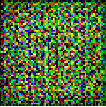

Discriminator

The DCGAN discriminator is a series of convolutional layers with leaky ReLU activation functions and batch normalization, designed to process 3-channel input images of size 64x64 pixels and output a single scalar value indicating the likelihood of the input image being real (1) or generated (0), using a sigmoid activation function to squash the output between 0 and 1.

D = nn.Sequential(
    # Input is 3 x 64 x 64 - Note RGB (vs Grayscale)
    nn.Conv2d(3, 64, (4, 4), (2, 2), (1, 1), bias=True),
    nn.LeakyReLU(0.2, True),
    # State size. 64 x 32 x 32
    nn.Conv2d(64, 128, (4, 4), (2, 2), (1, 1), bias=False),
    nn.BatchNorm2d(128),
    nn.LeakyReLU(0.2, True),
    # State size. 128 x 16 x 16
    nn.Conv2d(128, 256, (4, 4), (2, 2), (1, 1), bias=False),
    nn.BatchNorm2d(256),
    nn.LeakyReLU(0.2, True),
    # State size. 256 x 8 x 8
    nn.Conv2d(256, 512, (4, 4), (2, 2), (1, 1), bias=False),
    nn.BatchNorm2d(512),
    nn.LeakyReLU(0.2, True),
    # State size. 512 x 4 x 4
    nn.Conv2d(512, 1, (4, 4), (1, 1), (0, 0), bias=True),
    nn.Sigmoid()
).to(device) 

Training

The DCGAN is trained by iteratively updating the generator and discriminator networks, where the generator learns to produce realistic images from random noise, and the discriminator learns to distinguish between real and generated images, until reaching a stable equilibrium.

Setup

# Configurable variables
NOISE_DIMENSION = 100
GENERATOR_OUTPUT_IMAGE_SHAPE = 28 * 28 * 3
BATCH_SIZE = 128
LEARNING_RATE = 0.0001
NUM_EPOCHS = 5000

Training Loop

# Loss and optimizer
criterion = nn.BCELoss()
d_optimizer = optim.Adam(D.parameters(), lr=LEARNING_RATE)
g_optimizer = optim.Adam(G.parameters(), lr=LEARNING_RATE)

for epoch in range(0,NUM_EPOCHS):
    data_iterator = iter(celeba_dataloader)
    images = next(data_iterator)

    batch_size = images.size(0)
    #images = images.reshape(batch_size, -1).to(device)

    # Reshape the images to 2D with shape (batch_size, channels, height, width)
    images = images.view(-1, 3, image_size, image_size).to(device)

    # Labels for real and fake images
    real_labels = torch.ones(batch_size, 1).to(device)
    fake_labels = torch.zeros(batch_size, 1).to(device)


    # Training the discriminator
    # Real images
    outputs = D(images)
    d_loss_real = criterion(outputs.squeeze().unsqueeze(1), real_labels)
    real_score = outputs

    # Fake images
    # z = torch.randn(batch_size, NOISE_DIMENSION).to(device)
    z = torch.randn(batch_size, NOISE_DIMENSION, 1, 1).to(device)
    fake_images = G(z)
    outputs = D(fake_images.detach())
    d_loss_fake = criterion(outputs.squeeze().unsqueeze(1), fake_labels)
    fake_score = outputs

    # Total discriminator loss
    d_loss = d_loss_real + d_loss_fake

    d_optimizer.zero_grad()
    g_optimizer.zero_grad()
    d_loss.backward()
    d_optimizer.step()

    # Training the generator
    z = torch.randn(batch_size, NOISE_DIMENSION, 1, 1).to(device)
    fake_images = G(z)
    outputs = D(fake_images)
    g_loss = criterion(outputs.squeeze().unsqueeze(1), real_labels)

    d_optimizer.zero_grad()
    g_optimizer.zero_grad()
    g_loss.backward()
    g_optimizer.step()

    if epoch % 100 == 0:
        print(f"Epoch [{epoch+1}/{NUM_EPOCHS}], Step [{epoch}/{len(celeba_dataloader)}], "
              f"D_loss: {d_loss.item():.4f}, G_loss: {g_loss.item():.4f}, "
              f"D(x): {real_score.mean().item():.2f}, D(G(z)): {fake_score.mean().item():.2f}")


generaged_images = G(z)[0]
generated_image = generaged_images.permute(1, 2, 0).detach().cpu().numpy()
plt.imshow( generated_image )
plt.axis('off')
plt.savefig(f'dcgan_generated_image.png')
plt.close()

Output

After a few minutes the output will be saved. Not beautiful, but you can see that the result is moving towards a face (even if it does look a bit scary).

After 5000 epochs:

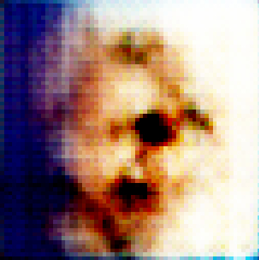
After 25000 epochs: